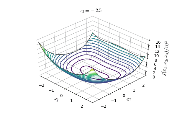
In mathematical optimization, the Rosenbrock function is really a non-convex function, created by Howard H. Rosenbrock in 1960, which is often used like a performance test problem for optimization algorithms. It’s also referred to as Rosenbrock’s valley or Rosenbrock’s blueberry function.
The worldwide minimum is in the lengthy, narrow, parabolic formed flat valley. To obtain the valley is trivial. To converge towards the global minimum, however, is tough.
The part is determined by
f
(
x
,
y
)
=
(
a
−
x
)
2
+
b
(
y
−
x
2
)
2
+b(y-x^)^
It features a global minimum at
(
x
,
y
)
=
(
a
,
a
2
)
)
, where
f
(
x
,
y
)
=
. These parameters are positioned so that
a
=
1
and
b
=
100
. Only within the trivial situation where
a
=
the part is symmetric and also the minimum reaches the foundation.
Two variants are generally experienced.
The first is the sum of the
N
/
2
uncoupled 2D Rosenbrock problems, and it is defined just for even
N
s:
This variant has predictably simple solutions.
Another, more involved variant is
has exactly one minimum for
N
=
3
(at
(
1
,
1
,
1
)
) and just two minima for
4
≤
N
≤
7
—the global the least all ones along with a local minimum near
(
x
1
,
x
2
,
…
,
x
N
)
=
(
−
1
,
1
,
…
,
1
)
,x_,dots ,x_)=(-1,1,dots ,1)
. This outcome is acquired by setting the gradient from the function comparable to zero, realizing the resulting equation is really a rational purpose of
x
. For small
N
the polynomials can be established exactly and Sturm’s theorem may be used to determine the amount of real roots, as the roots could be bounded around
x
i
<
2.4
x_